Assign fossil occurrences to spatial bins

A function to assign fossil occurrences (or localities) to spatial bins/samples using a hexagonal equal-area grid.

Usage

bin_space(
  occdf,
  lng = "lng",
  lat = "lat",
  spacing = 100,
  sub_grid = NULL,
  return = FALSE,
  plot = FALSE
)

Arguments

occdf

dataframe. A dataframe of the fossil occurrences (or localities) you wish to bin. This dataframe should contain the decimal degree coordinates of your occurrences, and they should be of class numeric.

lng

character. The name of the column you wish to be treated as the input longitude (e.g. "lng" or "p_lng").

lat

character. The name of the column you wish to be treated as the input latitude (e.g. "lat" or "p_lat").

spacing

numeric. The desired spacing between the center of adjacent cells. This value should be provided in kilometres.

sub_grid

numeric. For an optional sub-grid, the desired spacing between the center of adjacent cells in the sub-grid. This value should be provided in kilometres. See details for information on sub-grid usage.

return

logical. Should the equal-area grid information and polygons be returned?

plot

logical. Should the occupied cells of the equal-area grid be plotted?

Value

If the return argument is set to FALSE, a dataframe is returned of the original input occdf with cell information. If return is set to TRUE, a list is returned with both the input occdf and grid information and polygons.

Details

This function assigns fossil occurrence data into equal-area grid cells using discrete hexagonal grids via the h3jsr package. This package relies on Uber's H3 library, a geospatial indexing system that partitions the world into hexagonal cells. In H3, 16 different resolutions are available (see here). In the implementation of the bin_space() function, the resolution is defined by the user-input spacing which represents the distance between the centroid of adjacent cells. Using this distance, the function identifies which resolution is most similar to the input spacing, and uses this resolution.

Additional functionality allows the user to simultaneously assign occurrence data to equal-area grid cells of a finer-scale grid (i.e. a ‘sub-grid’) within the primary grid via the sub_grid argument. This might be desirable for users to evaluate the differences in the amount of area occupied by occurrences within their primary grid cells. This functionality also allows the user to easily rarefy across sub-grid cells within primary cells to further standardise spatial sampling (see example for basic implementation).

Note: prior to implementation, coordinate reference system (CRS) for input data is defined as EPSG:4326 (World Geodetic System 1984). The user should transform their data accordingly if this is not appropriate. If you are unfamiliar with working with geographic data, we highly recommend checking out Geocomputation with R.

Developer(s)

Lewis A. Jones

Reviewer(s)

Bethany Allen & Kilian Eichenseer

Examples

# Get internal data
data("reefs")

# Reduce data for plotting
occdf <- reefs[1:250, ]

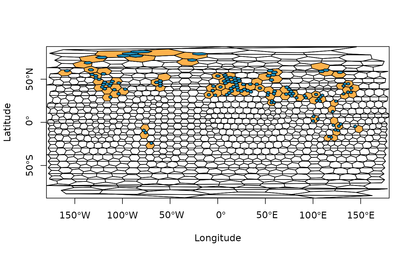
# Bin data using a hexagonal equal-area grid
ex1 <- bin_space(occdf = occdf, spacing = 500, plot = TRUE)
#> Average spacing between adjacent cells in the primary grid was set to 725.17 km. 
#> H3 resolution: 1

# Bin data using a hexagonal equal-area grid and sub-grid
ex2 <- bin_space(occdf = occdf, spacing = 1000, sub_grid = 250, plot = TRUE)

#> Average spacing between adjacent cells in the primary grid was set to 725.17 km. 
#> H3 resolution: 1

# EXAMPLE: rarefy
# Load data
occdf <- tetrapods[1:250, ]

# Assign to spatial bin
occdf <- bin_space(occdf = occdf, spacing = 1000, sub_grid = 250)
#> Average spacing between adjacent cells in the primary grid was set to 725.17 km. 
#> H3 resolution: 1

# Get unique bins
bins <- unique(occdf$cell_ID)

# n reps
n <- 10

# Rarefy data across sub-grid grid cells
# Returns a list with each element a bin with respective mean genus richness
df <- lapply(bins, function(x) {
  # subset occdf for respective grid cell
  tmp <- occdf[which(occdf$cell_ID == x), ]

  # Which sub-grid cells are there within this bin?
  sub_bin <- unique(tmp$cell_ID_sub)

  # Sample 1 sub-grid cell n times
  s <- sample(sub_bin, size = n, replace = TRUE)

  # Count the number of unique genera within each sub_grid cell for each rep
  counts <- sapply(s, function(i) {
    # Number of unique genera within each sample
    length(unique(tmp[which(tmp$cell_ID_sub == i), ]$genus))
  })

  # Mean richness across subsamples
  mean(counts)
})